Research
Research Topics
Developing Models for Advancing Ecology
Process Guided Deep Learning to Predict Dissolved Oxygen
Dissolved oxygen (DO) is a critical water quality constituent that governs habitat suitability for aquatic biota, biogeochemical reactions and solubility of metals in streams. While sensors have enabled the continuous monitoring of hundreds of streams for DO, there are still many more places where we have no data. With a team of USGS collaborators, I worked to build a data-driven model that can learn from the large volume of sensor data available while also leveraging our theoretical understanding of stream dissolved oxygen cycling. We incorporated the biological processes of photosynthesis and respiration into a machine learning model (LSTM) to predict dissolved oxygen concentrations in unmonitored river basins. This approach, which has been successfully used in other fields, is novel for water quality modeling. See our results so far: Sadler, Carter, et al. 2024. Hydrological Processes
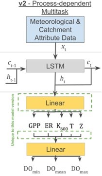
Conceptual schematic of the process-guided deep learning model used to predict stream DO concentrations. This model is a long short-term memory (LSTM) model that leverages information from previous time steps combined with model input data at the current time step to make predictions using a set of cell states (c), hidden states (h) and a linear output layer. This model used estimates of daily stream metabolism (the process driving oxygen concentration) to inform the model predictions. Figure from Sadler, Carter, et al. 2024. Hydrological Processes.
Sparse Modeling Approaches for Time Series Data
Long-term ecological datasets are valuable for understanding how ecosystems change over time and they are key to forecasting ecosystem responses to challenges like climate change and management actions. The value of long-term datasets is widely acknowledged, yet we still have limited methods for making full use of the growing volume of data, and the analytical methods for handling it are evolving. I am working with the Modelscapes Consortium to address these needs. In this project we aim to explore the application of Bayesian regularization and unsupervised learning methods to ecological time series.
Bayesian regularization of time series models can help to both select the most important predictors out of a wide range of explanatory variables, and bypass the steps needed and subjectivity involved in traditional time series analysis. Using regularization, or the shrinkage of parameters, models can learn which effects to include. We are testing the use of regularizing Bayesian priors for autoregressive AR(p) models to select among many covariates as well as a sparse vector of autoregressive (ф) coefficients.
Bayesian learning models may also be able to improve time series forecasts, even when little or no data are available on covariates. Many long-term datasets are cyclical and can be modeled as the sum of their underlying frequencies in the form of Fourier terms. By selecting only a few out of a large number of potential series using regularizing priors, we are working to generate robust forecasts with minimal explanatory variables. So far, our simulation models suggest that adding Gaussian priors has some effect on preventing overfitting and improving forecasts, and horseshoe priors improve models even more.
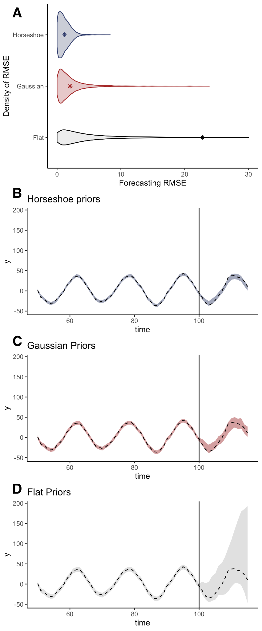
Forecasts from simulated time series using Bayesian sparse modeling methods with different prior probabilities on inclusion of predictors. Regularizing Horseshoe priors, or even Gaussian priors improve the forecasting ability of models by excluding spurious relationships, even when the predictors are correlated with each other. Figure from Gannon, Carter, et al. In prep.
Models for Missing Data in Ecology
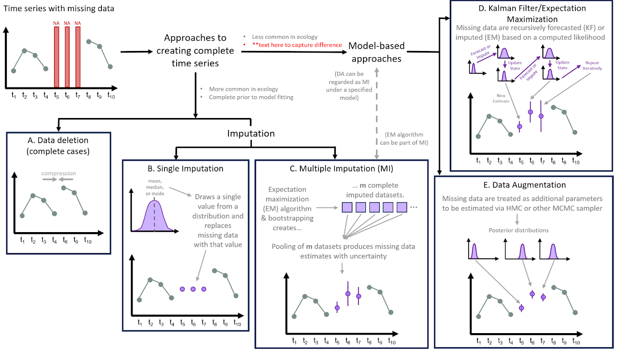
There are many different approaches to modeling time series with missing data, ranging from simple data deletion, to imputation techniques and model based approaches such as expectation maximization and Bayesian data augmentation. Figure from Stears, Carter, et al. In prep.
Missing data are the norm rather than the exception in ecology. Analyzing data with missing values can lead to biased estimates of parameters and reduced statistical power, leading to incorrect conclusions. This can be even more problematic in time series, where data are often both a response and a predictor, and a single missing observation can mean that we have to delete the subsequent time point as well because it is missing the predictor. For higher order AR models, this can result in large data gaps. As part of the Modelscapes Consortium, I am exploring methods to properly handle missing data in time series models. We are comparing how well models can recover parameters and fill in missing data points on simulated data with different mechanisms of missingness, including missing at random, autocorrelated missingness resulting in large gaps, and missing not at random.
River Ecosystem Energetics
Linking Carbon Fluxes to Biomass Building in Rivers
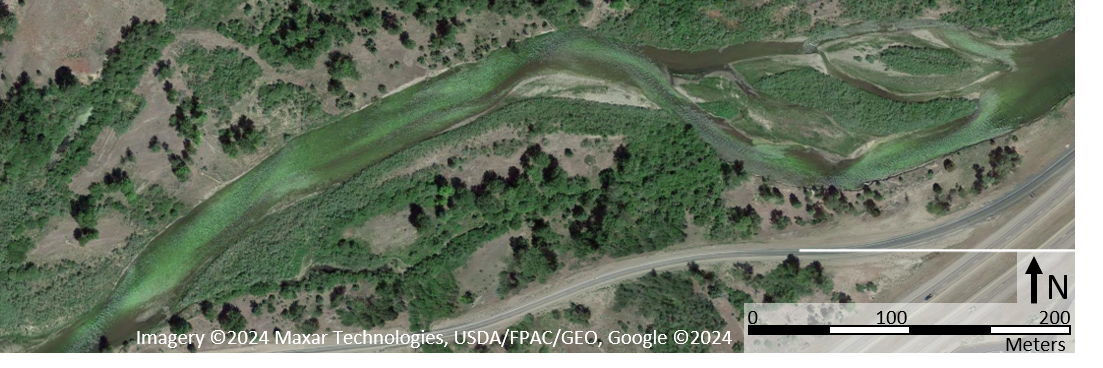
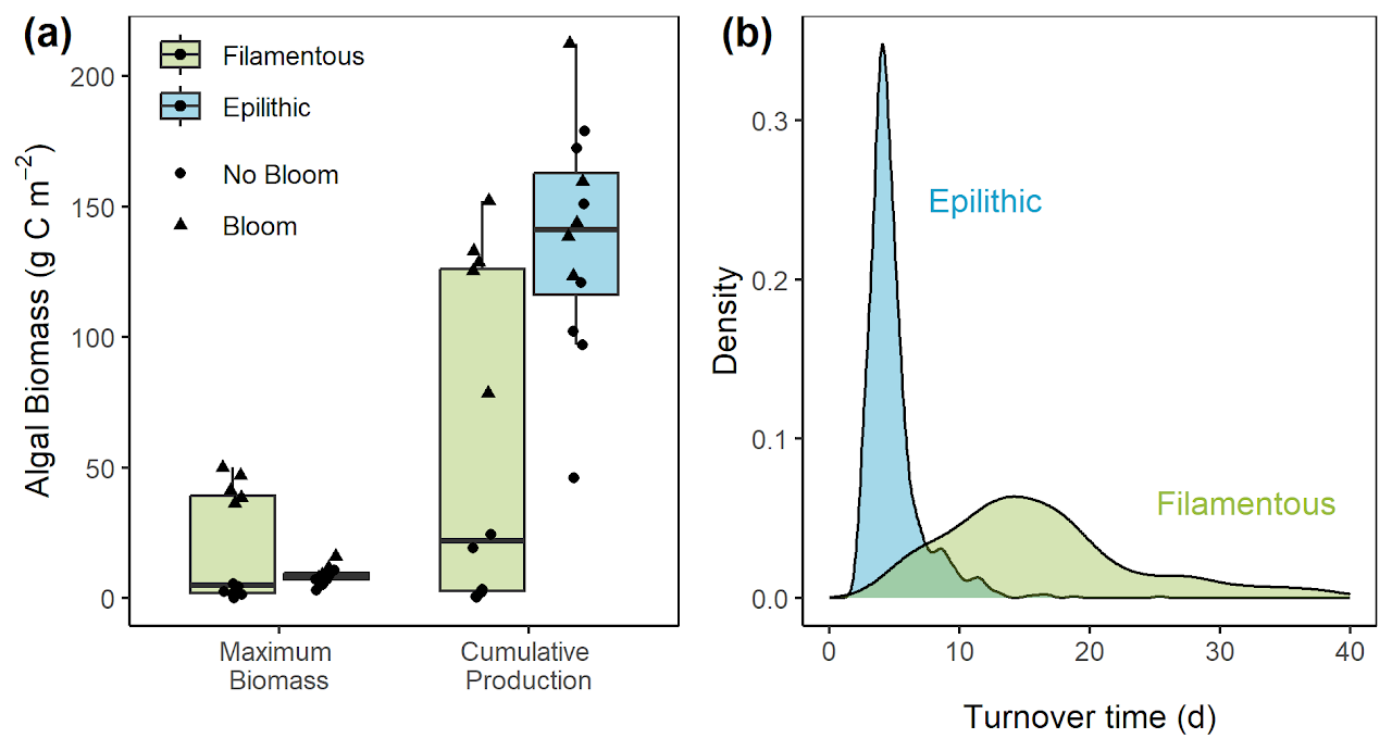
River ecosystems exert internal, biological control that mediates the effect of external drivers on carbon cycling. To understand these internal dynamics, I am studying the Upper Clark Fork River, an autotrophic river impaired by mine waste and nutrient pollution in Montana. The Clark Fork regularly experiences nuisance filamentous algae blooms that have been exacerbated by decades of ranching and agriculture in the watershed. I monitored the metabolism of the river in six different sites along a 120 km section to see if metabolism time series can reflect the presence of benthic algae blooms and shed light on the degree to which these blooms—internal biological control—mediate the effects of light and hydrology. I have found that time series models are better able to predict primary productivity if they incorporate information about the algal biomass and assemblage, indicating that the external controls are indeed, only part of the story.
We can partition the productivity time series across different algal forms (filamentous algae and thin epilithic biofilms) using a novel modeling approach that leverages the variability in algal distribution in space and time. By doing this, I found that despite large increases in biomass during algal blooms, the variation in growth forms of primary producers contributed little to the variation in ecosystem primary productivity. A small but rapidly cycling group of epilithic algae are the main contributors to ecosystem carbon cycling, while the slow growing filamentous algae dominate the carbon stocks.
This study links the structure and the function of stream primary producer communities and finds a somewhat surprising disconnect. Much of our fundamental understanding of this link comes from terrestrial ecosystem theory, but the departure we observe from this theory may be common in aquatic ecosystems.
Understanding Autotrophy in Rivers at a Continental Scale
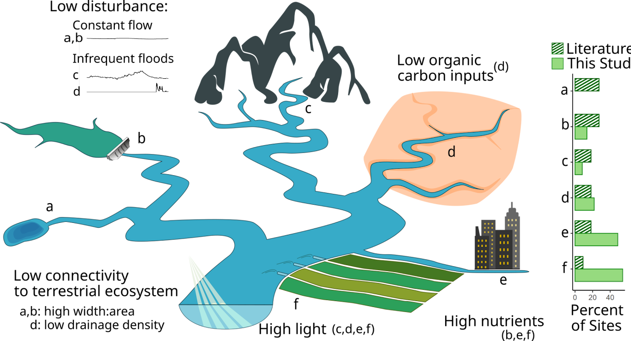
It is a long-standing paradigm in stream ecology that most streams are heterotrophic ecosystems, that is, they consume more organic carbon (supplied from terrestrial ecosystems) than they produce (through photosynthesis). However, autotrophic rivers have been observed across diverse landscapes where high light, low flow disturbance, and low organic carbon inputs are common. I led a team of limnologists to study how common autotrophy is, and what factors drive its occurrence using a dataset comprising 236 rivers and 921 years of daily metabolism. Because the possible number of watershed, climate, and in-stream covariates that could influence autotrophy is vast, this question is one of sparse data---meaning the number of potential predictors approaches the number of data points. We fit two versions of the regression model y = Xβ + ε, where autotrophy (y) is a function of a matrix of predictors (X) and a vector of coefficients (β) plus error (ε); first we constrained the potential predictors by only including the most important covariates as hypothesized based on a review of the literature on autotrophic streams. Second, we used a data-driven sparse model approach called Least Absolute Shrinkage and Selection Operator (LASSO). This regularization technique constrains the coefficients of a regression model by minimizing the loss function defined by L(β) = (y − Xβ)T(y − Xβ) + λ ∑ |βi|, where λ is a penalty parameter. This technique selects a subset of relevant covariates while shrinking most of the effects () to zero. Using this paired approach, we confirmed some of the hypothesized drivers while also finding new synthesis variables such as elevation that are useful in predicting autotrophy.
The Impact of Climate Change on River Carbon Cycling
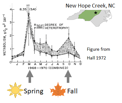
Much like forests, streams have annual ecosystem energy cycles. Stream algae and moss and other primary producers require light for photosynthesis, just like plants. In small streams, this means that peak productivity occurs in the early spring, before trees have all of their leaves that shade the stream. At the scale of a year, streams break down more organic carbon than they produce, and this additional fuel comes from plants and soils. In the fall, carbon consumption is high in streams as microbes and stream insects break down all of the leaves that fall from trees. Climate change is altering the timing and the rates of these fundamental ecosystem processes in streams. In my research, I am studying stream energetics in New Hope Creek, which is the site of the first ever study of annual stream energetics in 1972. This stream flows through a protected watershed in the Duke Forest, and little about it has changed in the fifty years since this foundational study except for the global change in climate leading to warmer water and more extreme floods and droughts. In comparison to fifty years ago, carbon and energy in New Hope Creek cycle faster, and hotter, drier falls have shifted the timing of most of this cycling. This means that organisms in the stream have less food available to them in the winter and that substantial release of greenhouse gasses and depletion of oxygen may become more common in the late summer and fall. This research demonstrates that changing climate will exacerbate the consequences to streams that we have observed in modified landscapes.
Past Research Projects
River Hypoxia
Hypoxia is when oxygen in an aquatic ecosystem is severely depleted, which can lead to fish kills, release of toxic metals from sediments, and production of atmospheric pollutants. Most research on hypoxia has focused on coastal areas and algal blooms in lakes, but in my research, I have observed extensive hypoxia throughout the rivers in the North Carolina Piedmont. My findings build on those from previous studies out of our research group that indicate that changes in river channel shape caused by urbanization including channel erosion from intense bursts of storm water flowing into culverts and flatter stream beds upstream of road impoundments are causing large portions of river networks to alternate between high storm flows and low flow leading to hypoxia.
Carter et al. 2021, Limnology and Oceanography · Blaszczak, Carter, et al. 2022, Limnology and Oceanography Letters
Greenhouse Gas Flux from Rivers
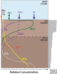
Most of the energy that fuels food webs in streams and rivers comes from breaking down plant matter and organic carbon that comes from outside of the ecosystem. The most efficient way to break down this carbon is using oxygen, through aerobic respiration. However, when oxygen is low, microbes can break down carbon through other, anaerobic metabolic pathways. Both aerobic and anaerobic respiration lead to the release of carbon dioxide into the atmosphere. Anaerobic pathways are additionally responsible for removal of reactive nitrogen through denitrification, the mobilization of heavy metals and contaminants, and release of organic carbon as methane, a potent greenhouse gas. When rivers are hypoxic, rates of anaerobic metabolism are high, but many observations indicate these pathways are active in the sediments even when the water column is oxygenated. In my research, I have found measurable rates of anaerobic metabolism at every location that I have looked for it.
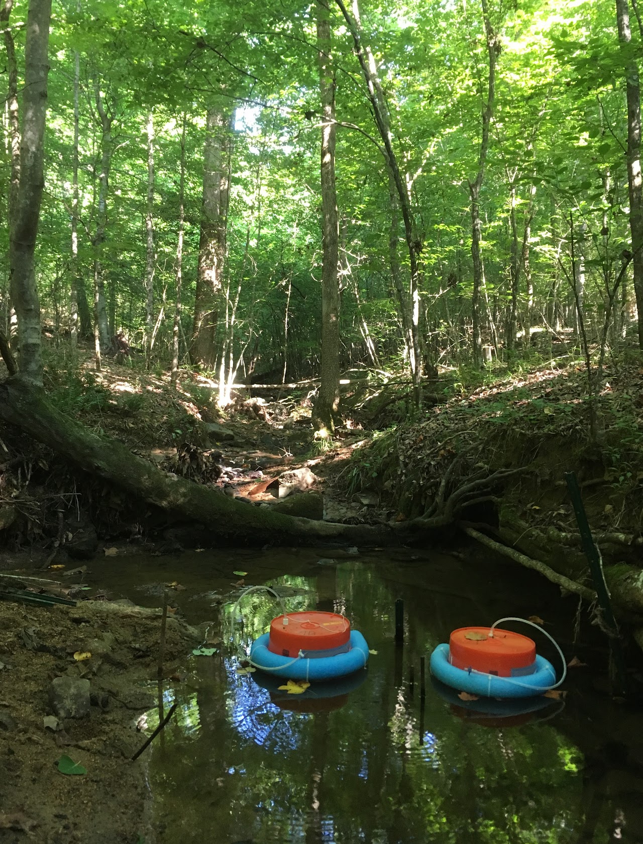
I am studying the release of greenhouse gasses, and the conditions that lead to this, in streams in Durham, North Carolina. I have found that flow and temperature both determine rates of carbon dioxide and methane production in streams. Importantly, human modification of river networks are creating conditions that deplete oxygen and favor anaerobic metabolism, resulting in more greenhouse gas pollution in the atmosphere.
Carter et al. 2022, JGR Biogeosciences · Delvecchia, Carter, et al. 2022, Limnology and Oceanography
Oceanic Flux Program at the Bermuda Institute for Ocean Sciences
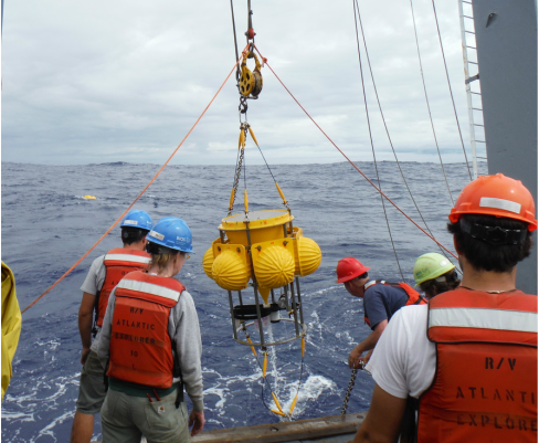
Before beginning work in streams, I worked with Dr. Maureen Conte as a research assistant for the Oceanic Flux Program. We worked to understand the rates and composition of oceanic particles that sink from the surface water, driving the distribution of organic matter and other elements in the deep ocean. Sinking particles undergo dynamic transformations as they are influenced by eddies and ocean currents, decomposition, secondary production and chemical processes. The particles that are observed at depth thus have a very complex temporal and chemical relationship with those formed in the surface ocean. I studied phosphorus phase partitioning and the trace element geochemistry of marine particles sinking through the water column at our field site in Bermuda. I found that iron and opal are important carriers of phosphorus to ocean sediments. Our research demonstrated that many trace elements have seasonal cycles at different depths in the ocean.
Toolik Lake Long Term Ecological Research Station
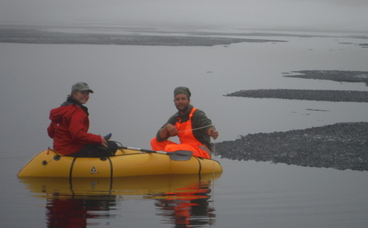
I worked under the guidance of Dr. Anne Giblin as the nutrient chemistry research assistant at Toolik Lake Long Term Ecological Research (LTER) site in northern Alaska. For two summers, I was part of a team conducting long term monitoring of Arctic lake ecosystems to understand how they respond to climate change and the nutrient loading that results when permafrost thaws.
Proyecto Costa Escondida — Sea Level Reconstruction in a Maritime Maya Site
The Proyecto Costa Escondida was an interdisciplinary team of geologists, ecologists and archeologists researching the occupation of an ancient Maya port city, Vista Alegre, on the Yucatan Peninsula in Mexico. I worked with hydrogeologist Dr. Patricia Beddows to reconstruct the patterns of sea level inundation in relation to the times of Maya inhabitation of the city. I analyzed sediment cores from shallow estuaries, constructing a stratigraphic record with δ¹⁸O and δ¹³C to look at sea level fluctuations during the Holocene. I found that periods of low sea-level indicated fresh water availability and correlated with times of site occupation by the Maya residents.